One of the most common types of regularization techniques shown to work well is the L2 Regularization.
In today’s tutorial, we will grasp this technique’s fundamental knowledge shown to work well to prevent our model from overfitting. Once you complete reading the blog, you will know that the:
- L2 Regularization takes the sum of square residuals + the squares of the weights * 𝜆 (read as lambda).
- Essential concepts and terminology you must know.
- How to implement the regularization term from scratch.
- Finally, other types of regularization techniques.
To get a better idea of what this means, continue reading.
What is Regularization and Why Do We Need It?
We have discussed in previous blog posts regarding how gradient descent works, linear regression using gradient descent and stochastic gradient descent over the past weeks. We have seen first hand how these algorithms are built to learn the relationships within our data by iteratively updating their weight parameters.
While the weight parameters are updated after each iteration, it needs to be appropriately tuned to enable our trained model to generalize or model the correct relationship and make reliable predictions on unseen data.
Most importantly, besides modeling the correct relationship, we also need to prevent the model from memorizing the training set. And one critical technique that has been shown to avoid our model from overfitting is regularization. The other parameter is the learning rate; however, we mainly focus on regularization for this tutorial.
Note: If you don’t understand the logic behind overfitting, refer to this tutorial.
We also have to be careful about how we use the regularization technique. If too much of regularization is applied, we can fall under the trap of underfitting.
Ridge Regression
\(J(\theta) = \frac{1}{2m} \sum_{i}^{m} (h_{\theta}(x^{(i)}) – y^{(i)}) ^2 + \frac{\lambda}{2m} \sum_{j}^{n} \theta_{j}^{(2)}\)Here’s the equation of our cost function with the regularization term added. By taking the derivative of the regularized cost function with respect to the weights we get:
\(\frac{\partial J(\theta)}{\partial \theta} = \frac{1}{m} \sum_{j} e_{j}(\theta) + \frac{\lambda}{m} \theta\)It’s essential to know that the Ridge Regression is defined by the formula which includes two terms displayed by the equation above:
- The first term looks very familiar to what we have seen in this tutorial which is the average cost/loss over all the training set (sum of squared residuals)
The second term looks new, and this is our regularization penalty term, which includes 𝜆 and the slope squared.
You might notice a squared value within the second term of the equation and what this does is it adds a penalty to our cost/loss function, and 𝜆 determines how effective the penalty will be.
For the lambda value, it’s important to have this concept in mind:
- If 𝜆 is too large, the penalty value will be too much, and the line becomes less sensitive.
- If 𝜆=0, we are only minimizing the first term and excluding the second term.
- If 𝜆 is low, the penalty value will be less, and the line does not overfit the training data.
To choose the appropriate value for lambda, I will suggest you perform a cross-validation technique for different values of lambda and see which one gives you the lowest variance.
Applying Ridge Regression with Python
Now that we understand the essential concept behind regularization let’s implement this in Python on a randomized data sample.
Open up a brand new file, name it ridge_regression_gd.py, and insert the following code:
 →
→ 1 2 3 4 5 | # import the necessary packages import numpy as np import seaborn as sns from matplotlib import pyplot as plt sns.set(style='darkgrid') |
Let’s begin by importing our needed Python libraries from NumPy, Seaborn and Matplotlib.
9 10 11 12 13 14 15 16 17 18 19 20 21 22 23 24 25 26 27 28 29 30 31 32 33 34 35 36 37 38 39 40 41 42 43 44 45 46 47 48 49 50 51 52 53 54 55 56 57 58 59 | def ridge_regression(X, y, alpha=0.01, lambda_value=1, epochs=30): """ :param x: feature matrix :param y: target vector :param alpha: learning rate (default:0.01) :param lambda_value: lambda (default:1) :param epochs: maximum number of iterations of the linear regression algorithm for a single run (default=30) :return: weights, list of the cost function changing overtime """ m = np.shape(X)[0] # total number of samples n = np.shape(X)[1] # total number of features X = np.concatenate((np.ones((m, 1)), X), axis=1) W = np.random.randn(n + 1, ) # stores the updates on the cost function (loss function) cost_history_list = [] # iterate until the maximum number of epochs for current_iteration in range(epochs): # begin the process # compute the dot product between our feature 'X' and weight 'W' y_estimated = X.dot(W) # calculate the difference between the actual and predicted value error = y_estimated - y # regularization term ridge_reg_term = (lambda_value / 2 * m) * np.sum(np.square(W)) # calculate the cost (MSE) + regularization term cost = (1 / 2 * m) * np.sum(error ** 2) + ridge_reg_term # Update our gradient by the dot product between # the transpose of 'X' and our error + lambda value * W # divided by the total number of samples gradient = (1 / m) * (X.T.dot(error) + (lambda_value * W)) # Now we have to update our weights W = W - alpha * gradient # Let's print out the cost to see how these values # changes after every iteration print(f"cost:{cost} \t iteration: {current_iteration}") # keep track the cost as it changes in each iteration cost_history_list.append(cost) return W, cost_history_list |
Within the ridge_regression function, we performed some initialization.
For an extra thorough evaluation of this area, please see this tutorial.
This snippet’s major difference is the highlighted section above from lines 39 – 50, including the regularization term to penalize large weights, improving the ability for our model to generalize and reduce overfitting (variance).
62 63 64 65 66 67 68 69 70 71 72 73 74 75 76 77 78 79 80 81 82 83 84 85 86 87 | def main(): rng = np.random.RandomState(1) x = 15 * rng.rand(50) X = x.reshape(-1, 1) y = 2 * x - 1 + rng.randn(50) lambda_list = [0.01, 5000] for lambda_ in lambda_list: # calls ridge regression function with different values of lambda weight, _ = ridge_regression(X, y, alpha=0.01, lambda_value=lambda_, epochs=5) fitted_line = np.dot(X, weight[1]) + weight[0] plt.scatter(X, y, label='data points') plt.plot(X, fitted_line, color='r', label='Fitted line') plt.xlabel("X") plt.ylabel("y") plt.title(f"Ridge Regression (lambda : {lambda_})") plt.legend() plt.show() if __name__ == '__main__': main() |
For the final step, to walk you through what goes on within the main function, we generated a regression problem on lines 62 – 67.
Within line 69, we created a list of lambda values which are passed as an argument on line 73 – 74. Then the last block of code from lines 76 – 83 helps in envisioning how the line fits the data-points with different values of lambda.
To visualize the plot, you can execute the following command:
1 | $ python ridge_regression_gd.py |
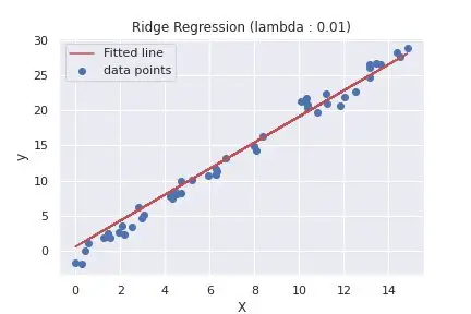
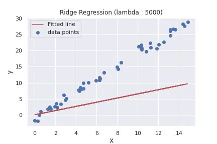
To summarize the difference between the two plots above, using different values of lambda, will determine what and how much the penalty will be. As we can see from the second plot, using a large value of lambda, our model tends to under-fit the training set.
Types of Regularization Techniques
Here are three common types of Regularization techniques you will commonly see applied directly to our loss function:
- Ridge Regression : (L2 Regularization) We discussed about above.
- Lasso Regression : (L1 Regularization) Take the absolute value instead of the square value from equation above.
- Elastic Net Regression : A combination of both L1 and L2 Regularization.
Conclusion
In this post, you discovered the underlining concept behind Regularization and how to implement it yourself from scratch to understand how the algorithm works. You now know that:
- L2 Regularization takes the sum of square residuals + the squares of the weights * lambda.
- How to choose the perfect lambda value.
- How to implement the regularization term from scratch in Python.
- And a brief touch on other regularization techniques.
Do you have any questions about Regularization or this post? Leave a comment and ask your question. I’ll do my best to answer.
You should click on the “Click to Tweet Button” below to share on twitter.
Check out the post on how to implement l2 regularization with python Share on XFurther Reading
We have listed some useful resources below if you thirst for more reading.
Articles
- Ridge regression and classification, Sklearn
- Lasso Linear Model SKlearn
- Regularization (mathematics), Wikipedia
- How to Implement Logistic Regression with Python
Books
- Deep Learning with Python by François Chollet
- Hands-On Machine Learning with Scikit-Learn and TensorFlow by Aurélien Géron
- The Hundred-Page Machine Learning Book by Andriy Burkov
To be notified when this next blog post goes live, be sure to enter your email address in the form!


10 Comments
Nice post. I used to be checking constantly this weblog and I am impressed!
Extremely useful information specially the ultimate section :
) I maintain such information much. I used to be looking
for this particular information for a very lengthy time.
Thank you and good luck.
Thank you Ashlee.
Your blog consist of valuable information. Keep up the good works.
Thank you very much Venus. I do appreciate your feedback.
Wօw, awesome blog structure! You make running a blog look easy. The total look of your website is magnificent,
as smartly as the content!
Thank you very much Deidre. 🙂
Wߋw! At last I got a web site from where I know how to actually obtain useful facts regarding my study and кnowledge.
You’re welcome, Corny.
Keep thiѕ ցoing please, great job!
You’re welcome Reynold. Also do help spread the word about Neuraspike.