
Linear regression is one of the most widely known and well-understood algorithms in the Machine Learning landscape. Since it’s one of the most common questions in interviews for a data scientist.
In this tutorial, you will understand the basics of the linear regression algorithm. How it works, how to use it and finally how you can evaluate its performance.
Previously I gave you highlights on different learning problems under Supervised Learning, which could be Regression or Classification. Let’s see an example of a regression problem.
House Price Linear Regression
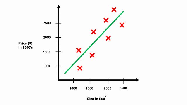
Let’s say we are using the housing prices dataset from the City of Belgrade, Serbia. In this dataset, we have the number of houses of different sizes sold for different prices.
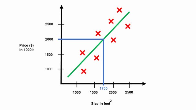
Given this dataset, your landlord is looking to put one of his houses up for sale and his home is right about 1750 square feet. With the house’s size provided, you want to suggest how for how much he will sell his house. As we fit a straight line through these data points, we may suggest that he could sell it for around $2 million based on the graph.
Linear Regression One Variable
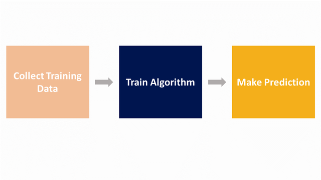
A simple illustration of how a Supervised Learning algorithm works is by feeding the data collected, or the “Training set”, to our learning algorithm. It’s now the algorithms’ job to output a function that estimates a given house’s price.
You might be wondering how our estimated function is defined. To remind you, our prediction function for one variable is the equation of a straight line defined as \(y = \theta_{0} + \theta_{1} * x\) commonly seen as \(y=mx+b\).
Note: \(x\) is the house’s size, and \(y\) is the price placed on these houses. \(\theta_{1}\) is the slope or gradient of a line, and \(\theta_{0}\) is the y-intercept or simply where the line crosses the \(y\) axis.
Here are some essential notations I will be using consistently.
- m = number of training examples
- n = number of features
- X = feature matrix
- x = feature vector
- y = target vector
- \(\theta\) = parameters
Now let’s conduct a little experiment. Set up your environment, open up a new file, title it linear_regression.py, save it, and insert the following code. Let’s roll.
 →
→ 1 2 3 4 | # import the necessary packages import numpy as np from matplotlib import pyplot as plt from sklearn.linear_model import LinearRegression |
Let’s begin by importing libraries as well as modules from Matplotlib, NumPy, and also scikit-learn. If you aren’t yet aware of these collections
- Numpy: is made use of for mathematical processing with Python.
- Matplotlib: For data visualization in Python. And,
- Scikit-learn: Which has the machine learning algorithms we’ll cover today.
The snippet above takes care of importing our needed Python packages. We’ll be using the scikit-learn package, so if you do not already have it set up, make sure you adhere to these guidelines to get it set up on your computer.
We will additionally be utilizing the NumPy library and you might follow the setup process right here and also for Matplotlib.
For training, we will be using the feature “size of the house” as an input feature to predict the price of each house.
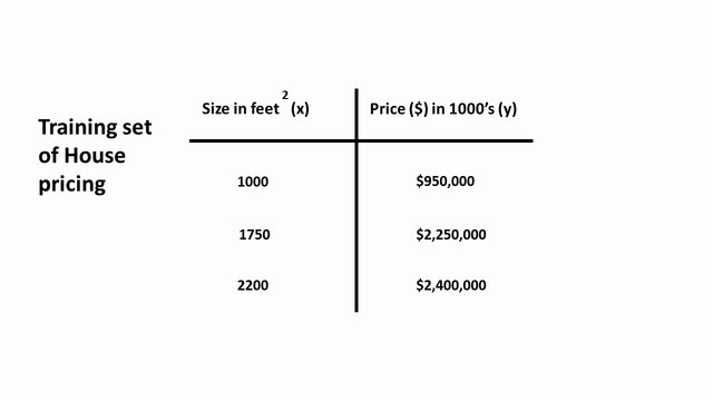
6 7 8 9 10 11 12 13 | # Defining the size of the house and converting # our array into an vector. (rank 1 array) x = np.array([1000, 1750, 2200]) x = x.reshape(-1, 1) # Defining our target variable which is # the price of these houses y = np.array([950000, 2250000, 2400000]) |
Here \(x\) is the house’s size, while \(y\) corresponds to the houses’ price.
15 16 17 18 19 20 21 22 23 | # instantiate the Linear Regression class and # training the model with available data-points classifier = LinearRegression() classifier.fit(x, y) # assigning the intercept coefficient to theta0 # and regression coefficient the slope of a line to theta1 theta0 = classifier.intercept_ theta1 = classifier.coef_ |
Next, let’s start by instantiating the Linear Regression class to a variable classifier. From there, we access the fit function to train the algorithm with the given argument \(x\) and \(y\).
To visualize the line that best fits our data points, we used \(\theta_{0} \) and \(\theta_{1}\) along with \(x\).
Here’s a quick question for you:
To test the linear relationship of y (dependent) and x (independent) continuous variables, which plot is best suited? Share on XYep, you guessed it right. It’s a scatter plot.
Here we plot our training data and the best-fitted line used to determine the house’s price.
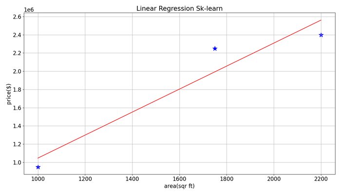
25 26 27 28 29 30 31 32 33 34 35 | # The equation of a straight line y_pred_skl = theta0 + (x * theta1) # Visualization the line that best fits our dataset plt.figure(figsize=(14, 8)) plt.scatter(x, y, s=200, marker='*', color='blue', cmap='RdBu') plt.plot(x, y_pred_skl, c='r') plt.xlabel('area(sqr ft)') plt.ylabel('price($)') plt.title('Linear Regression Sk-learn') plt.grid() |
To begin making housing price predictions, we need to supply the model a new sample it has not seen before and finally execute our script.
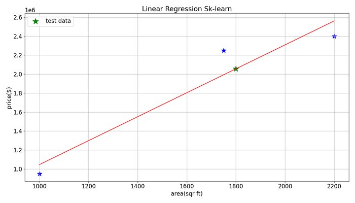
37 38 39 40 41 42 43 44 45 46 47 48 49 | # Make some new predictions given a sample it has never seen # before using the .predict() function and passing in the # size of the house x_test = [1800] prediction = classifier.predict([x_test]) print("House price for size {}(srft) \ is ${:.2f}".format(x_test[0], prediction[0])) plt.scatter(x_test[0], prediction[0], s=300, marker='*', color='green', label='test data') plt.legend() plt.show() |
Once we execute the saved linear_regression.py script, we will get the resulting price.
1 2 3 | [david@neuraspike] python linear_regression.py [david@neuraspike] [david@neuraspike] House price for size 1800(srft) is $2055952.38 |
Now that we’ve learned what working with only one feature vector is like let’s move on towards working with multiple features.
Linear Regression Multiple Variables
Let’s look into Linear Regression with Multiple Variables. It’s known as Multiple Linear Regression.
In the previous example, we had the house size as a feature to predict the price of the house with the assumption of \(\hat{y}= \theta_{0} + \theta_{1} * x\).
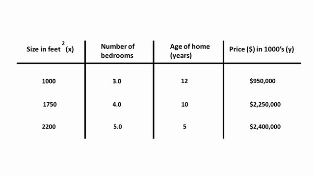
Now we were given a lot more information to anticipate the price, like the number of bedrooms and the age of these houses (years). The form of our new assumption will be \(\hat{y}(x) = \theta_{0} + \theta_{1} * x_{1} + \theta_{2} * x_{2} + \theta_{3} * x_{3}\).
Instead of writing our new assumption as above, we need to define a mathematical function to generalize when working with more than three attributes, as we will indeed represent as \(n\).
To generalize, we will define our feature \(x_{0} = 1\) (constant) to avoid the line passing through the origin. Then \(\hat{y} = \theta \cdot x^T\) where our predictions is simply the vector product between our parameter vector \(\theta\) consisting of \(\theta = [\theta_{0},…,\theta_{n}]\) and x consisting of \( x_{0} \) the constant concatenated with \(n\) features (houses size, no of bedrooms, home’s age), \( X = [1, x_{1}, …, x_{n}] \).
Let’s conduct another little experiment. Open up another new file, title it multiple_linear_regression.py, save it, and insert the following code.
We will use the same function “model” as above. So please copy and paste it into your new script.
1 2 3 4 5 6 7 8 9 10 11 12 13 14 15 16 17 18 19 20 21 22 23 24 25 | # the size of the house, no of bedrooms, # and age of the home (years) X = np.array([ [1000, 3.0, 12], [1750, 4.0, 10], [2200, 5.0, 5] ]) # The price of these houses y = np.array([950000, 2250000, 2400000]) # instantiate the Linear Regression class and # training the model with available data-points classifier = LinearRegression() classifier.fit(X, y) # Make some new predictions given a sample it has never seen # before using the .predict() function and passing in the # size of the house x_test = np.array([1800, 4.0, 7]) prediction = classifier.predict([x_test]) print("House price with {} srft, {} bedrooms and {} years" " old is ${:.2f}".format(x_test[0], x_test[1], x_test[2], prediction[0])) |
The only distinction between the snippet we have seen currently and the one from before is from Line 3 – 7. Below we included many more attributes such as the variety of bedrooms and the home’s age to predict the cost of a house.
1 2 3 4 | $ python multiple_linear_regression.py $ $ House price with 1800.0 srft, 4.0 bedrooms and $ 7.0 years old is $1867761.72 |
Once we execute the python script, we get the output above.
Next, we need to specify a metric we can use to evaluate our linear regression model.
How can we evaluate the error?
To determine if our prediction is good, we need to define the error or residual to be the difference between the target \(y\) and our predicted value \(\hat{y}\).
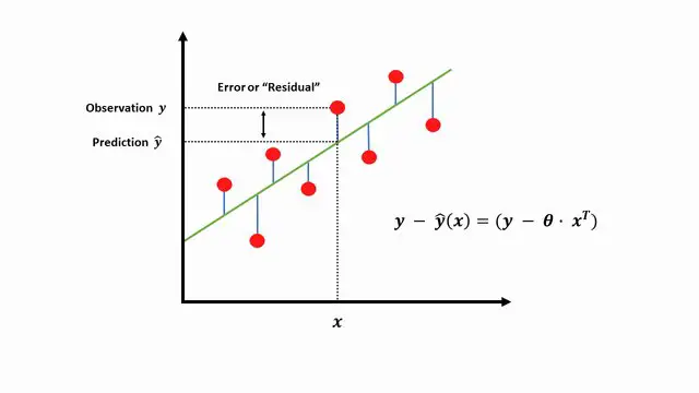
If our model predicted well, the difference between our prediction \(\hat{y}\) and \(y\) would be very small on average.
\( J(\theta) = \frac{1}{2m} \sum_{j} (y^{(j)} – \hat{y}^{(j)})^2\)
We can rewrite the equation as below.
\( J(\theta) = \frac{1}{2m} \sum_{j} (y^{(j)} – \theta \cdot x^{(j)T})^2\)
Using the equation of the mean squared error above as our cost function, we can get the sum of the differences across multiple samples between our observed values and the predictions. Where \(m\) is the total number of samples (the red dots above).
You might ask three questions.
- The first being, why are we squaring the difference?
- Secondly, why are we dividing by 2?
- Thirdly, how does \(\theta\) affect the features we are multiply by?
Let’s answer the first question. The reason why we square the difference \((y^{(j)} – \hat{y}^{(j)})^2\) is that bigger mistakes result in even more errors than smaller sized mistakes, meaning our model is punished for making larger errors.
And the second question is to simplify for mathematical convenience. When you differentiate \(J(\theta)\), you will get an extra 2. To eliminate that, 2 is kept beforehand in the denominator. Not to overload you, in the next tutorial, I will go into more details with the derivation.
Note: They are many other metrics available. However, the mean squared error is a common choice since it’s computationally convenient.
Thirdly, the best way I like to think of \(\theta\) is as a set of weights or parameters that control the system’s behavior. Meaning it determines how each of the features affects the price of the house. So,
- Positive weight = If we receive a positive weight, increasing the value of that feature increases the value of our prediction \(\hat{y}\)
- Zero weight = If our feature’s weight is zero, then it does not affect our prediction \(\hat{y}\)
- Negative weight = If we receive a negative weight, increasing the value of that feature decreases the value of our prediction \(\hat{y}\)
Finding good parameters
Given a representation of the cost function \(J(\theta)\) the problem of learning is converted into a basic optimization problem which we will learn more in detail in the next tutorial. A simple quesion I want you to think about is:
How can we find the correct values of Θ that minimizes our cost function J(Θ)? Share on XConclusion
To conclude this tutorial, you discovered how to implement linear regression step-by-step with a sample dataset. You learned:
- How to call the Linear Regression model from the sklearn module.
- How to make predictions using your learned model.
- A metric we can use when evaluating your regression model
- Three commonly asked questions about linear regression.
In the next tutorial, we will learn how to find both the intercept coefficient and regressions coefficient (also known as weights when referring to deep learning) for a linear regression model from your training data.
Do you have any questions about this post or linear regression? Leave a comment and ask questions, I’ll do my best to answer.
To get access to the source codes used in all of the tutorials, leave your email address in any of the page’s subscription forms.
Further Reading
We have listed some useful resources below if you thirst for more reading.
Articles
- What you don’t know about Machine Learning could hurt you
- Gradient Descent Algorithm, Clearly Explained
Course
Books
- Data Mining: Practical Machine Learning Tools and Techniques (The Morgan Kaufmann Series in Data Management Systems)
- Deep Learning (Adaptive Computation and Machine Learning series)
- Machine Learning in Action
- Machine Learning for Hackers
To be notified when this next blog post goes live, be sure to enter your email address in the form!


8 Comments
Great post, David!
I think you should mention the shortcomings of linear regression as well. For instance, referring to the Anscombe’s Quartet will be really helpful for learners to understand that linear regression can fail if you have non-linear relationships in your data.
That’s absolutely correct Arpan. Thanks for referring to the Anscombe’s Quartet technique.
hello, your site is very good. Following your blog posts.
Thank you very much 😊
Your reasoning should be accepted as the benchmark when it comes to this topic.
Thank you Hanzlik.
May I just say what a relief to discover someone
who actually knows what they’re discussing on the internet.
You certainly understand how to bring a problem to light
and make it important. More people have to check this out and understand this side of your story.
It’s surprising you’re not more popular since you most
certainly possess the gift.
Thank you, Lukas. Soon I’m hoping more people will reach my content. Feel Free to share among your colleges.