In today’s tutorial, we will learn about the basic concept of another iterative optimization algorithm called the stochastic gradient descent and how to implement the process from scratch. You will also see some benefits and drawbacks behind the algorithm.
If you aren’t aware of the gradient descent algorithm, please see the most recent tutorial before you continue reading.
The Concept behind Stochastic Descent Descent
One of the significant downsides behind the gradient descent algorithm is when you are working with a lot of samples. You might be wondering why this poses a problem.
The reason behind this is because we need to compute first the sum of squared residuals on as many samples, multiplied by the number of features. Then compute the derivative of this function for each of the features within our dataset. This will undoubtedly require a lot of computation power if your training set is significantly large and when you want better results.
Considering that gradient descent is a repetitive algorithm, this needs to be processed for as many iterations as specified. That’s dreadful, isn’t it? Instead of relying on gradient descent for each example, an easy solution is to have a different approach. This approach would be computing the loss/cost over a small random sample of the training data, calculating the derivative of that sample, and assuming that the derivative is the best direction to make gradient descent.
Along with this, as opposed to selecting a random data point, we pick a random ordering over the information and afterward walk conclusively through them. This advantageous variant of gradient descent is called stochastic gradient descent.
In some cases, it may not go in the optimal direction, which could affect the loss/cost negatively. Nevertheless, this can be taken care of by running the algorithm repetitively and by taking little actions as we iterate.
Applying Stochastic Gradient Descent with Python
Now that we understand the essentials concept behind stochastic gradient descent let’s implement this in Python on a randomized data sample.
Open a brand-new file, name it linear_regression_sgd.py, and insert the following code:
 →
→ 1 2 3 4 5 6 | # import the necessary packages from matplotlib import pyplot as plt import seaborn as sns import numpy as np sns.set(style='darkgrid') |
Let’s get started by importing our required Python libraries from Matplotlib, NumPy, and Seaborn.
9 10 11 12 13 14 15 16 17 18 19 20 21 | def next_batch(features, labels, batch_size): """ :param features: feature matrix :param labels: target vector :param batch_size: size of mini-batch :return: a list of the current batched features and labels """ # iterate though a mini batch of both our features and labels for data in range(0, np.shape(features)[0], batch_size): # append the current batched features and labels in a list yield (features[data: data+batch_size], labels[data: data+batch_size]) |
To correctly apply stochastic gradient descent, we need a function that returns mini-batches of the training examples provided. This next_batch function takes in as an argument, three required parameters:
- Features:
The feature matrix of our training dataset. - Labels: The class labels link with the training data points.
- batch_size: The portion of the mini-batch we wish to return.
Along with this, the batch size is set to one by default. Nonetheless, we commonly make use of mini-batches that are greater than one.
Note: A few other values include 32, 64, 128, and 256.
So, why are these numbers the typical mini-batch size standard? Making use of a batch size greater than one does help reduce the difference (variance) in the parameter update and helps bring about a more stable convergence.
26 27 28 29 30 31 32 33 34 35 36 37 38 39 40 41 42 43 44 | def stochastic_gradient_descent(X, y, alpha=0.01, epochs=100, batch_size=1): """ :param X: feature vector :param y: target vector :param alpha: learning rate (default=0.01) :param epochs: maximum number of iterations of the linear regression algorithm for a single run (default=100) :param batch_size: the portion of the mini-batch (default=1) :return: weights, list of cost function changing overtime """ m = np.shape(X)[0] # total number of samples n = np.shape(X)[1] # total number of features X = np.concatenate((np.ones((m, 1)), X), axis=1) W = np.random.randn(n + 1, ) # stores the updates on the lost/cost function cost_history_list = [] |
Within the stochastic_gradient_descent function, we performed some initialization.
For an extra thorough evaluation of this area, please see last week’s tutorial.
Now below is our actual Stochastic Gradient Descent (SGD) implementation in Python:
46 47 48 49 50 51 52 53 54 55 56 57 58 59 60 61 62 63 64 65 66 67 68 69 70 71 72 73 74 75 76 77 78 79 80 81 82 83 84 85 86 | # iterate until the maximum number of epochs for current_iteration in range(epochs): # begin the process # save the total lost/cost during each batch batch_epoch_loss_list = [] for (X_batch, y_batch) in next_batch(X, y, batch_size): # current size of the feature batch batch_m = np.shape(X_batch)[0] # compute the dot product between our # feature 'X_batch' and weight 'W' y_estimated = X_batch.dot(W) # calculate the difference between the actual # and estimated value error = y_estimated - y_batch # get the cost (Mean squared error -MSE) cost = (1 / 2 * m) * np.sum(error ** 2) batch_epoch_loss_list.append(cost) # save it to a list # Update our gradient by the dot product between the # transpose of 'X_batch' and our error divided by the # few number of samples gradient = (1 / batch_m) * X_batch.T.dot(error) # Now we have to update our weights W = W - alpha * gradient # Let's print out the cost to see how these values # changes after every each iteration print(f"cost:{np.average(batch_epoch_loss_list)} \t" f" iteration: {current_iteration}") # keep track of the cost cost_history_list.append(np.average(batch_epoch_loss_list)) # return both our weight and list of cost function changing overtime return W, cost_history_list |
Let’s start by looping through our desired number of epochs.
Next, to keep track of the cost throughout each batch processing, let’s initialize a batch_epoch_cost_list, which we will certainly use to calculate the average loss/cost over all mini-batch updates for each epoch.
Within the inner loop exists our stochastic gradient descent algorithm. The significant difference between what we discovered last week, and what you are reading currently, is that we aren’t going over all our training samples at once. We are looping over these samples in mini-batches as explained above.
For each mini-batch returned to us by the next_batch function, we take the dot product between our feature matrix and weights matrix. Then compute the error between the estimated value and actual value.
When we evaluate the gradient for the current batch, we have the gradient which can then update the weight matrix \(W\) by simply multiplying the gradient scaled by the learning rate subtracted from the previous weight matrix.
Again, for a more thorough, detailed explanation of the gradient descent algorithm, please see last week’s tutorial.
If you are having difficulties understanding the concept behind gradient descent, please refer to this tutorial.
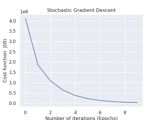
89 90 91 92 93 94 95 96 97 98 99 100 101 102 103 104 105 106 107 108 109 | def main(): rng = np.random.RandomState(10) X = 10 * rng.rand(1000, 5) # feature matrix y = 0.9 + np.dot(X, [2.2, 4., -4, 1, 2]) # target vector # calls the stochastic gradient descent method weight, cost_history_list = stochastic_gradient_descent(X, y, alpha=0.001, epochs=10, batch_size=32) # visualize how our cost decreases over time plt.plot(np.arange(len(cost_history_list)), cost_history_list) plt.xlabel("Number of iterations (Epochs)") plt.ylabel("Cost function J(Θ)") plt.title("Stochastic Gradient Descent") plt.show() if __name__ == '__main__': main() |
For the final step, to walk you through what goes on within the main function, where we generated a regression problem, on lines 90 – 92. We have a total of 1000 data points, each of which is 5D.
Our main objective is to correctly map these randomized feature training samples \((1000×5)\) (a.k.a dependent variable) to our independent variable \((1000×1)\).
On lines 95-98, we pass the feature matrix, target vector, learning rate, number of epochs, and the batch size to the stochastic_gradient_descent function, which returns the best parameters and the saved history of the lost/cost after each iteration.
The last block of code from lines 101 – 105 aids in envisioning how the cost adjusts on each iteration.
To check the cost modifications from your command line, you can execute the following command:
1 2 3 4 5 6 7 8 9 | $ python linear_regression_sgd.py $ $ cost:5499006.995697101 iteration: 0 $ cost:2521982.7383839684 iteration: 1 $ cost:1485829.8191042473 iteration: 2 ... $ cost:109915.08892952456 iteration: 7 $ cost:66752.14911602132 iteration: 8 $ cost:41288.896510311075 iteration: 9 |
Advantages of Stochastic Gradient Descent
Usually in practice, stochastic gradient descent is often preferred if we have:
- Lots of data: Stochastic gradient descent has better speed properties because we don’t have to touch all \(m\) datapoints before updating our \(\theta\) parameter once.
- Computationally fast: Updating our parameter is done quickly after seeing a few data points before modifying it.
Drawbacks of Stochastic Gradient Descent
Nonetheless, since the procedure is random, it can be:
- Harder to Debug: Difficulty in assessing convergence.
- Harder to know when to stop: Stopping conditions may be harder to evaluate.
Feel free to click the “Click to Tweet” button if you enjoyed the post.
Check out the post on Stochastic Gradient Descent (SGD) with Python. Share on XConclusion
To conclude this tutorial, you learned about Stochastic Gradient Descent (SGD), a common extension to the gradient descent algorithm in today’s blog post. You’ll see SGD used in nearly all situations instead of the original gradient descent version. You learned:
- The Concept behind Stochastic Descent Descent Algorithm
- How to Apply the Algorithm yourself in Python
- Benefits of using the Algorithm
- Then a few drawbacks behind the Algorithm
Do you have any questions about this post or Stochastic Gradient Descent? Leave a comment and ask your question. I’ll do my best to answer.
To get access to the source codes used in all of the tutorials, leave your email address in any of the page’s subscription forms.
Reference
Further Reading
We have listed some useful resources below if you thirst for more reading.
Course
Books
- Data Mining: Practical Machine Learning Tools and Techniques (The Morgan Kaufmann Series in Data Management Systems)
- Machine Learning for Hackers
- Applied Predictive Modeling
To be notified when this next blog post goes live, be sure to enter your email address in the form!


6 Comments
Very nice post. I just stumbled upon your weblog and wished to say that I have really enjoyed surfing around your
blog posts. In any case I will be subscribing to your mailing list feed and I hope you write again soon!
Thank you very much, Stephany.
I just like the helpful information you supply in your articles.
I’ll bookmark your blog and take a look at again right here regularly.
I am slightly certain I’ll be told many new stuff proper right here!
Best of luck for the next!
Thank you Veola.
This is a topic that i love so much. Thank you for this tutorial.
You are welcome Jarrod.