In the last two tutorials, I have specified the equation of the mean squared error \(J(\theta)\), which measures how wrong the model is in modeling the relationship between \( X \) and \( y \).
In continuation of the previous tutorial behind the gradient descent algorithm, you will undoubtedly learn how to perform linear regression using gradient descent in Python on a new cost function \( J(\theta) \) the “mean square error”.
Not only will you get a greater understanding of the algorithm, which I had guaranteed, yet additionally execute a Python script yourself.
First, let’s review some ideas concerning the topic.
Gradient Descent Review
What we want to achieve is to update our \( \theta \) value in a way that the cost function gradually decreases over time.
To accomplish this, what should we do actually? This is a specific questions we have to decide on. Should we reduce or increase the values of \( \theta \) ?
Considering the graph, we must take a step in the negative direction (going downwards).
Every step we take always provides us a new value of \( \theta \). When we obtain a new value, we need to constantly keep track of the gradient, and evaluate it gradient with newfound value, then repeat taking the same step until we are at the global minimum (the blue dot).
Gradient Descent Illustration
A straightforward illustration of the gradient descent algorithm is as follow:
1 2 3 4 5 6 | Initialize theta # keep updating our theta values while we haven't converged do { theta = theta - alpha * J(theta) } while(Not converged) |
- Initialization: We initialize our parameters \( \theta \) arbitrarily.
- Iteration: Then iterate finding the gradient of our function \( J(\theta) \) and updating it by a small learning rate, which may be constant or may change after a certain number of iterations.
- Stopping: Stopping the procedure either when \( J(\theta) \) is not changing adequately or when our gradient is sufficiently small.
Gradient For The Mean Squared Error (MSE)
\( J(\theta) = \frac{1}{2m} \sum_{j} (\theta x^{(j)} – y^{(j)})^ 2 \) [1.0]
For linear regression, we can compute the Mean Squared Error cost function and then compute its gradient.
\( J(\theta) = \frac{1}{2m} \sum_{j} (\theta_{0}x_{0}^{(j)} \hspace{2mm} + \hspace{2mm} \theta_{1}x_{1}^{(j)} \hspace{2mm} + \hspace{2mm} … \hspace{2mm} \theta_{n}x_{n}^{(j)} – y^{(j)})^ 2 \) [1.1]
Let’s expand our prediction right into each term and currently signify the error residual \( e_{j}(\theta) \) to simplify the way we will write it.
\( e_{j}(\theta) \) as \( (\theta_{0}x_{0}^{(j)} \hspace{2mm} + \hspace{2mm} \theta_{1}x_{1}^{(j)} \hspace{2mm} + \hspace{2mm} … \hspace{2mm} \theta_{n}x_{n}^{(j)} \hspace{2mm} – \hspace{2mm}y^{(j)}) \)
Taking the derivative of this equation sounds a little more tricky if you’ve been out of calculus class for a while. However, don’t stress too much. I’ve got you covered. Let’s begin by showing you the derivation procedure.
\(\frac{\partial J(\theta)}{\partial \theta} = \frac{ \partial}{\partial \theta} \frac{1}{2m} \sum_{j} e_{j}(\theta)^2\) [1.2]
\(\frac{\partial J(\theta)}{\partial \theta} = \frac{1}{2m} \sum_{j} \frac{\partial}{\partial \theta} e_{j}(\theta)^2\) [1.3]
To move from formula [1.2] to [1.3], we need to use two necessary derivative regulations. The scalar multiple and sum rule:
Scalar multiple rule: \(\hspace{10mm} \frac{d}{dx} (\alpha \hspace{0.3mm} u) = \alpha \frac{du}{dx}\)
Sum rule: \( \hspace{10mm} \frac{d}{dx} (\sum \hspace{0.3mm} u) = \sum \frac{du}{dx}\)
\(\frac{\partial J(\theta)}{\partial \theta} = \frac{1}{2m} \sum_{j} \hspace{1mm} 2 e_{j} \hspace{1mm}(\theta) \hspace{1mm} \frac{\partial}{\partial \theta} \hspace{1mm} e_{j}(\theta)\) [1.4]
Next what we did to get from [1.3] to [1.4], is we applied both the power rule and the chain rule. If you’re not accustomed to the guidelines, you may discover them below:
Power rule: \(\hspace{10mm} \frac{d}{dx} u ^n = nu^{n-1} \frac{du}{dx}\)
Chain rule: \(\hspace{10mm} \frac{d}{dx} f(g(x)) = {f}'(g(x)) \hspace{1mm}{g}'(x)\)
\(\frac{\partial J(\theta)}{\partial \theta} = \frac{1}{m} \sum_{j} e_{j}(\theta)\) [1.5]
Lastly, to go from [1.4] to [1.5], equation [1.5] gives us the partial derivative of the MSE \(J(\theta)\) with respect to our \(\theta\) variables.
We can assess by taking the partial derivative of the Mean Squared Error (MSE) with respect to \(\theta_{0}\).
\( \frac{\partial}{\partial \theta_{0}} e_{j}(\theta) = \frac{\partial}{\partial \theta_{0}} \theta_{0}x_{0}^{(j)} + \frac{\partial}{\partial \theta_{0}} \theta_{1}x_{1}^{(j)} + …. + \frac{\partial}{\partial \theta_{0}} \theta_{n}x_{n}^{(j)} \hspace{1mm} – \hspace{1mm} y^{(j)}= x_{0}^{(j)} \)To find the given partial derivative of the function, we should deal with the other variables as constants. Such as when taking this partial derivative of \(\theta_{0}\), all other variables are dealt with as constants \(( y, \theta_{1}, x_{1}, …, x_{n} )\).
We can duplicate this for various other parameters like \(\theta_{1}, \theta_{2} …. \theta_{n} \) and instead of just attribute \(x_{0}^{j}\) we will obtain features \(x_{1}^{j}, x_{2}^{j}, … ,x_{n}^{j}\).
Applying Gradient Descent in Python
Now we know the basic concept behind gradient descent and the mean squared error, let’s implement what we have learned in Python.
Open up a new file, name it linear_regression_gradient_descent.py, and insert the following code:
 →
→ 1 2 3 4 5 6 | # import the necessary packages from matplotlib import pyplot as plt import numpy as np import seaborn as sns sns.set(style='darkgrid') |
Let’s start by importing our required Python libraries from Matplotlib, NumPy, and Seaborn.
9 10 11 12 13 14 15 16 17 18 19 20 21 22 23 24 25 26 | def gradient_descent(X, y, alpha=0.01, epochs=30): """ :param x: feature matrix :param y: target vector :param alpha: learning rate (default:0.01) :param epochs: maximum number of iterations of the linear regression algorithm for a single run (default=30) :return: weights, list of the cost function changing overtime """ m = np.shape(X)[0] # total number of samples n = np.shape(X)[1] # total number of features X = np.concatenate((np.ones((m, 1)), X), axis=1) W = np.random.randn(n + 1, ) # stores the updates on the cost function (loss function) cost_history_list = [] |
Next, let’s arbitrarily initialize and concatenate our intercept coefficient and regression coefficient represented by \(W\) “weights.”
One thing that might puzzle you by now is, why initialize our weights arbitrarily? Why not establish it as all 0’s or 1’s?
The reason behind this logic is because:
- If the weights in our network start too small, then the output shrinks until it’s too small to be useful.
- If the weights in our network start too large, then the output swells until it’s too large to be useful.
So we intend to set it at about a suitable value because we want to calculate interesting functions.
Once those values have been initialized arbitrarily, let’s define some constants based on the size of our Dataset and an empty list to keep track of the cost function as it changes each iteration.
- n : The overall number of samples
- cost_history_list : Save the history of our cost function over after every iteration (at some point described as epochs)
28 29 30 31 32 33 34 35 36 37 38 | # iterate until the maximum number of epochs for current_iteration in range(epochs): # begin the process # compute the dot product between our feature 'X' and weight 'W' y_estimated = X.dot(W) # calculate the difference between the actual and predicted value error = y_estimated - y # calculate the cost (Mean squared error - MSE) cost = (1 / 2 * m) * np.sum(error ** 2) |
While iterating, until we reach the maximum number of epochs, we calculate the estimated value y_estimated which is the dot product of our feature matrix \(X\) as well as weights \(W\).
With our given predictions, the following step is to determine the “error” or merely the difference between our actual value “y” and our estimated value “y_estimated.” Then evaluate our prediction with the overall performance of the machine learning model for the given training data with a set of weights initialized to get the cost.
40 41 42 43 44 45 46 | # Update our gradient by the dot product between # the transpose of 'X' and our error divided by the # total number of samples gradient = (1 / m) * X.T.dot(error) # Now we have to update our weights W = W - alpha * gradient |
The next action will be to calculate the partial derivative with respect to the weights \(W\). When we have the gradient, we need to readjust the previous values for \(W\). That is, the gradient multiplied by the learning rate alpha deducted from the previous weight matrix.
48 49 50 51 52 53 54 55 56 | # Let's print out the cost to see how these values # changes after every 10th iteration if current_iteration % 10 == 0: print(f"cost:{cost} \t iteration: {current_iteration}") # keep track the cost as it changes in each iteration cost_history_list.append(cost) return W, cost_history_list |
A condition statement is being utilized to print out how the cost function changes every 10 epochs on the console.
To keep track of exactly how the cost function changes over time, we include the values into a list cost_history_list on each iteration. Then return our parameters \(W\) and cost_history_list populated with the changes in our cost function over time.
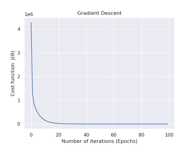
59 60 61 62 63 64 65 66 67 68 69 70 71 72 73 74 75 76 | def main(): rng = np.random.RandomState(10) X = 10 * rng.rand(100, 5) # feature matrix y = 0.9 + np.dot(X, [2.2, 4., -4, 1, 2]) # target vector # calls the gradient descent method weight, cost_history_list = gradient_descent(X, y, alpha=0.01, epochs=100) # visualize how our cost decreases over time plt.plot(np.arange(len(cost_history_list)), cost_history_list) plt.xlabel("Number of iterations (Epochs)") plt.ylabel("Cost function J(Θ)") plt.title("Gradient Descent") plt.show() if __name__ == '__main__': main() |
For the final step, to walk you through what goes on within the main function, we generated a regression problem on lines 60 – 62. We have a total of 100 data points, each of which are 5D.
Our goal is to correctly map these randomized feature training samples \((100×5)\) (a.k.a. dependent variable) to our independent variable \((100×1)\).
Within line 65, we pass the feature matrix, target vector, learning rate, and the number of epochs to the gradient_descent function, which returns the best parameters and the saved history of the lost/cost after each iteration.
The last block of code from lines 68 – 72 aids in envisioning how the cost adjusts on each iteration.
To check the cost modifications from your command line, you can execute the following command:
1 2 3 4 5 6 7 8 9 | $ python linear_regression_gradient_descent.py $ $ cost:2870624.491941226 iteration: 0 $ cost:145607.02085484721 iteration: 10 $ cost:17394.518134046495 iteration: 20 ... $ cost:72.96453135073557 iteration: 70 $ cost:71.71480871397247 iteration: 80 $ cost:70.89080664015975 iteration: 90 |
Observations on Gradient Descent
In my view, gradient descent is a practical algorithm; however, there is some information you should know.
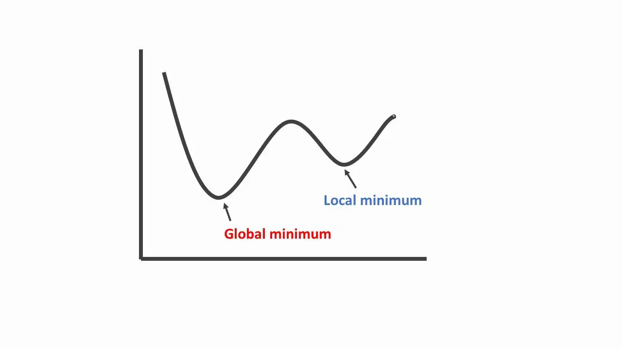
- Local Minima: It can be sensitive to initialization and can get stuck in local minima. Meaning, depending on the value given to \(\theta\) it will give us a different gradient direction leading either towards a local or global minimum.
- Step Size: The selection of step size can influence both the convergence rate and our procedure’s behavior. If the chosen step size is too large, we can jump over the minimum, and if it’s too small, we make very little progress increasing the amount of time it takes to converge.
Conclusion
To conclude this tutorial, you discovered how to implement linear regression using Gradient Descent in Python. You learned:
- An easy brush up with the concept behind Gradient Descent.
- How to calculate the derivative of the mean squared error.
- How to implement Linear Regression using Gradient Descent in Python.
- Observations behind the gradient descent algorithm.
Do you have any questions concerning this post or gradient descent? Leave a comment and ask your question. I’ll do my best to answer.
To get access to the source codes used in all of the tutorials, leave your email address in any of the page’s subscription forms.
You should click on the “Click to Tweet Button” below to share on twitter.
Check out the post on Linear Regression using Gradient Descent (GD) with Python. Share on XFurther Reading
We have listed some useful resources below if you thirst for more reading.
Course
Articles
- Intro to optimization in deep learning: Gradient Descent
- Why Initialize a Neural Network with Random Weights?
Books
To be notified when this next blog post goes live, be sure to enter your email address in the form!


18 Comments
Please let me know the link to the source code of this article. I will be thankful.
To get all access to the source code used in all tutorials, leave your email address in any of the page’s subscription forms.
Great info. I’ve been seeking for this content.
Thank you very much Alex.
Heya i’m for the first time here. I found your blog and I find It really useful & it helped me out a lot.
I hope to give something back and help others like you helped me.
It’s my pleasure Chelsey.
Ӏ waѕ able to find good info from your content.
It’s honestly my pleasure Arnulfo.
Incredible points. Sound arguments. Keep up the amazing effort.
Thank you very much Mohammed for your kind feedback.
Hello
Thank you very much for your super useful tutorial. I just don’t get how you move from equation 1.4 to 1.5, could you explain it to me please ?
Thanks again
Xavier
Since the value 2 is a constant, it is brought outside of the summation sign. Then, we will have (2*1) / (2*m), which can be simplified into 1/m.
Hi there! Someone in my Facebook group shared this website with us so I came to look it over.
I’m definitely loving the information. I’m bookmarking and will be tweeting this
to my followers! Terrific blog and amazing style and design.
Thank you very much, Benny, for your kind words, and I appreciate your honest feedback. Stay tuned for more tutorials on the blog, and don’t forget to subscribe to my Youtube channel, as I recently started releasing a bunch of video tutorials.
Youtube Channel: https://www.youtube.com/channel/UCsbZWuMs4rzTwjzNGa9JrqA
Hi, I do not understand how this calculates the gradient:
gradient = (1 / m) * X.T.dot(error)
Is the gradient just as simple as the dot product of the features and the error?
How is the gradient the same size as W. Let’s say you have 2 features and 4 samples, X is 4×2 matrix, and the error is 1×4. The gradient would be a 1×2. What if our W is of any size other than that?
Hello Saleh, and thanks for asking your question.
Yes, the gradient is simply the dot product between the features matrix (Transposed) and the error (the squared difference between the actual label and predicted value).
Regarding your question about whether the calculation is possible if W (the weighted matrix) is of any size. Well, if could be as long as this rule when performing matrix multiplication hold which states:
– Two matrices can be multiplied only when the number of columns in the first equals the number of rows in the second.
If the statement doesn’t hold, then it’s not possible.
Hi, I have some questions
1. How do you make sure the gradient is the same size as W. Shouldn’t every gradient[i] correspond to the weight W[i]?
gradient = (1 / m) * X.T.dot(error)
Lets say there are 4 samples and 2 features, so X is a 4×2 matrix. The error is 1×4. The gradient would be 1×2. But what if W is another size?
Thanks again, Saleh, for asking your question.
We used vectorization to speed up the Python code without using for loop (np.dot() method). Which will help minimize the runtime of our code, making it much efficient.
I’ll strongly recommend you implement for yourself the same procedure using Python for loop and time how long each operation takes the run, using a larger matrix.
A great way to assert if “X” and “W” are the exact sizes, is to use the assert keyword available in Python.