How to Estimate the Bias and Variance with Python

A helpful way of comprehending, underfitting and overfitting is as a balance between bias and variance.

In today’s tutorial, we will learn about some machine learning fundamentals, which are bias and variance. How to estimate a given model’s performance using the California housing dataset with Python, and finally, how to tackle overfitting/underfitting.

The Conceptual Definition between Bias and Variance​

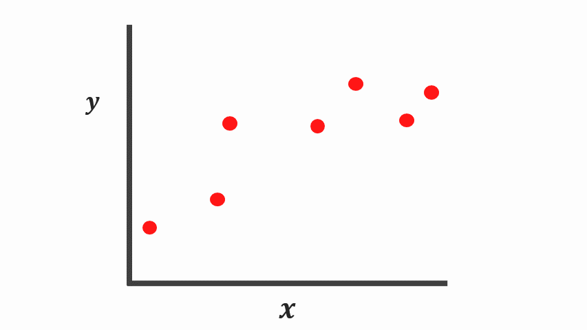
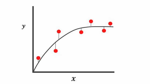
Let’s say we are given a simple regression problem with one feature \(X\) and a real value target \(y\), and we want to learn the relationship between \(X\) and \(y\). In this instance, we aren’t sure about the appropriate formula to approximate the relationship well enough. So let’s come up with two different machine learning methods.

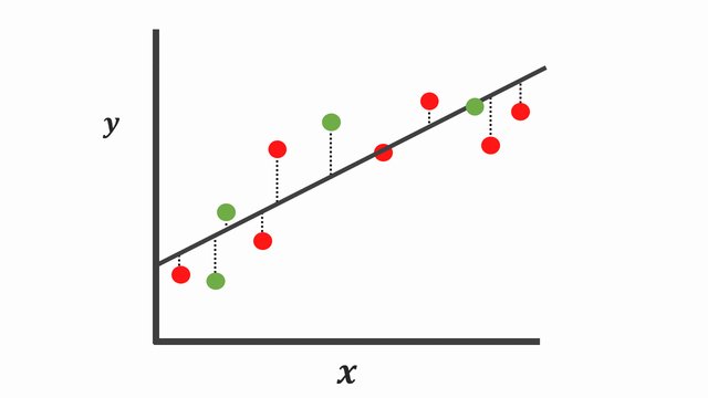
The first method is to fit a simple linear regression (simple model) through the data points   \(y=mx+b+e\).  Note the \(e\) is to ensure our data points are not entirely predictable, given this additional noise.

And on the other hand, another very different explanation of the same data points is a complex function since the line touches all these data points exactly.

Taking a look at the graphs, it’s arguable both of these models explain the data points properly using different assumptions.

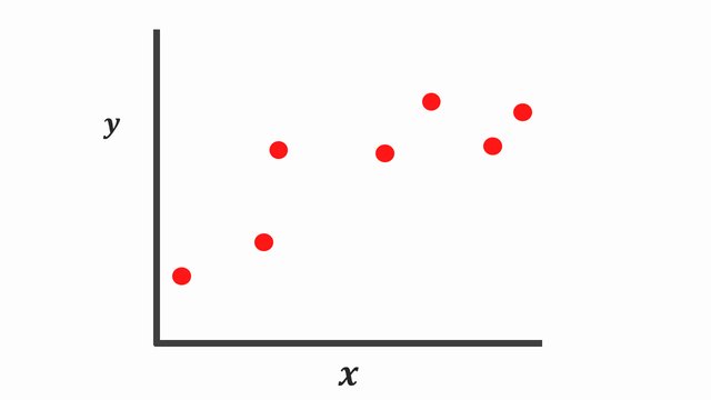
However, the real test is not how well these assumptions described the relationship during the training time, yet how well they perform on unseen data points.

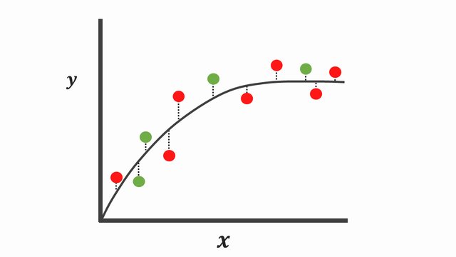
When we collect and expose both assumptions defined to some new collections of data points colored in green, we can see our first assumptions still performs well even when we calculate the sum of squares for the testing set.

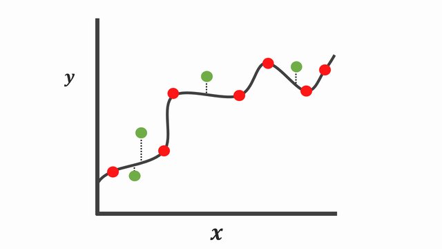
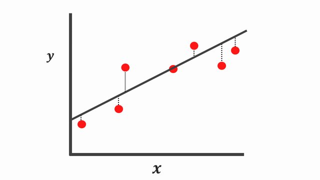
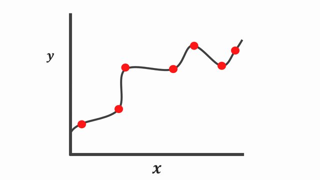
On the contrary, the complex function [Figure 5] fits the training data points so well that this complex curve poorly explains many of these points during the testing phase. Although this complex curve explains all the data points seen during the training phase, it tends to exhibit low properties on data that is hasn’t seen before. Typically referred to as overfitting.

As we might have seen from the plot above [Figure 5], the complex curve has low bias since it correctly models the relationship between \(X\) and \(y\). However, this isn’t appropriate cause it has high variability. Besides, when you compute the loss/cost or sums of squares for new data points, the difference will be a lot. And if we choose to make future predictions with this model, the results might be useful sometimes, and another time, it will perform terribly.

Instead, using a simple model [Figure 4] tends to have a high bias due to its inability to capture the true relationship between \(X\) and \(y\).  It’s important to know there is low variance because when we compute the sum of squares residuals, the difference isn’t that much. And occasionally, we could get good predictions and other times, not so great predictions.

In the Machine Learning dialect, since the curve fits the training data points well and not the testing points, we can conclude the curved line overfits. Then, on the other hand, if the line doesn’t fit the training well and does for the testing points, we say the curved line underfits.

What is the bias-variance Trade-off?

When building any supervised machine learning algorithm, an ideal algorithm should have a relatively low bias that can accurately model the true relationship among training samples,

and low variability, by producing consistent predictions across data points it hasn’t seen before. However, this poses a challenge due to the following:

• Reducing the bias will surely increase the variance.
• Decreasing the variance of the model will undoubtedly increase bias.

It’s important to know they are a trade-off between these two concepts, and the goal is to balance or achieve a sweet spot (optimum model complexity) between these two concepts that would not underfit or overfit.

How to Estimate the Bias and Variance with Python

Now we know the standard idea behind bias, variance, and the trade-off between these concepts, let’s demonstrate how to estimate the bias and variance in Python with a library called mlxtend.

This unbelievable library created by Sebastian Raschka provides a bias_variance_decomp() function that can estimate the bias and variance for a model over several samples. This function includes the following parameters:

• estimator : A regressor or classifier object that performs a fit or predicts method similar to the scikit-learn API.​
• X_train : The training dataset dataset
• y_train : The targets that correspond with the X_train examples
• X_test : The test dataset used for computing the average loss, bias, and variance that corresponds with the X_train examples
• y_test : The targets that correspond with the y_test examples
• loss : The loss function for performing the bias-variance decomposition. Only compose of ‘0-1_loss’ and ‘mse’
• num_rounds : Total number of rounds for performing the bias-variance decomposition
• random_seed : Used to initialize a pseudo-random number generator for the bias-variance decomposition

To get started, let’s first install this library. Fire up your command line and type in the following command:

Or to install using conda:

As soon as that’s complete, open up a brand new file, name it estimate_bias_variance.py, and insert the following code:

→ Click here to download the code

Let’s begin by importing our needed Python libraries from Sklearn, NumPy, and our lately installed library, mlxtend.

Next, let’s fetch the California housing dataset from the sklearn API. After that split the data into a training and testing set.

To approximate the average expected loss (mean squared error) for linear regression, the average bias and average variance for the model’s error over 50 bootstrap samples.

Once we execute the script, we will get an average expected loss, bias, and variance of the model errors.
When running the algorithm, the results printed out on the console changes once you re-run the script. So at least take the average of all the outputs to come to a reasonable conclusion.

To interpret what you see at the output, we are given a low bias and low variance using a linear regression model. Also, the sum of the bias and variance equals the average expected loss.

How to Tackle Under/Overfitting

You can tackle underfitting by performing the following operations:

• Add more features, parameters.
• Deceasing Regularization terms, which I will talk about in the next tutorial
• Use more complex models. For example, when using a straight line, add polynomial features.

You can tackle overfitting by performing the following operations:

• Removing features forcing our model to underperform to avoid overfitting
• Increase the Regularization terms / Adding some early stopping technique
• Use a less complex model
• Include more training data

Conclusion

In this post,  you discovered the concept behind bias and variance. You also learned how to estimate these values from your machine learning model, and finally, how to tackle overfitting/underfitting in machine learning.

You learned:

• Bias is the assumptions made by the model that causes it to over-generalize and underfit your data.
• Variance is how much the target function will change while been trained on different data.
• The bias-variance trade-off is simply the balance between the bias and variance to ensure that our model generalizes on the training data and performs well on the unseen data.

Do you have any questions about bias or variance? Leave a comment and ask your question. I’ll do my best to answer.

You should click on the “Click to Tweet Button” below to share on twitter.

Credit

• Raschka, Sebastian (2018) MLxtend: Providing machine learning and data science utilities and extensions to Python’s scientific computing stack.
  

Further Reading

We have listed some useful resources below if you thirst for more reading.

Articles

• Linear Regression using Stochastic Gradient Descent in Python
  
• Understanding the Bias-Variance Tradeoff
  
• Bias-Variance Decomposition
  
• Bias–variance tradeoff, wikipedia
  

Books

• Deep Learning with Python by François Chollet
  
• Hands-On Machine Learning with Scikit-Learn and TensorFlow by Aurélien Géron
  
• The Hundred-Page Machine Learning Book by Andriy Burkov
  

To be notified when this next blog post goes live, be sure to enter your email address in the form!