The common question you usually hear is, is Logistic Regression a Regression algorithm as the name says?
Last week I decided to run a poll over Twitter about the Logistic Regression Algorithm, and around 64.1% of the audience got the answer correctly.
In today’s tutorial, we will grasp this fundamental concept of what Logistic Regression is and how to think about it. We will also see some mathematical formulas and derivations, then a walkthrough through the algorithm’s implementation with Python from scratch. Finally, some pros and cons behind the algorithm.
To get a better understanding, continue reading.
Before continuing with the tutorial, yesterday was my birthday, and I love to thank everyone who sent birthday wishes. If you would like to support me on this cheerful day, and share the joy, I accept all kinds of gifts, God bless.
What is Logistic Regression?
As the name states, it’s one of the most poorly named algorithms in the field of machine learning. By thinking of the name, you might assume it’s one of the regression methods. However, this isn’t true. It’s a classification method.
Other than what I’ve mentioned don’t be confused, it’s one of the most widely used classification algorithms in medicine, for instance, if a patient is likely to die due to some particular pathological state. In finance, if a bank will lose a customer due to the services provided, etc.
Lastly, what I love about Logistic Regression is that, not only is it a classification method, yet, it builds perfect knowledge of what neural networks are, which we will discuss in future tutorials.
The intuition behind Logistic Regression
Before going into the tech talk behind the algorithm, let’s walk you through an example. Let’s say you want to build a machine learning model to predict if a customer is likely to cancel their monthly subscription based on the services provided to them. Having a solution is crucially vital for large subscription businesses to identify customers most at-risk of churning.
Now we want to model the probability (churn | x) “the probability the customer is likely to churn given some data about the person.
Let’s say this \( X \) feature matrix consist of \( x_{1}\) which is the person’s age, \(x_{2}\) = monthly charges given to a person, \(x_{3}\) = internet speed plan offered. Now taking a linear combination of these feature variables provided gives us
\( w_{0}x_{0} + w_{1}x_{1} + w_{2}x_{2} + w_{3}x_{3} = W^{T} X \)by transforming it into a vector where \( X = [1, x1, x2, x3] \)
The main issue behind the formula we have modeled above is, it isn’t a probability. It’s merely a plane, as we have seen in the tutorials related to linear regression.
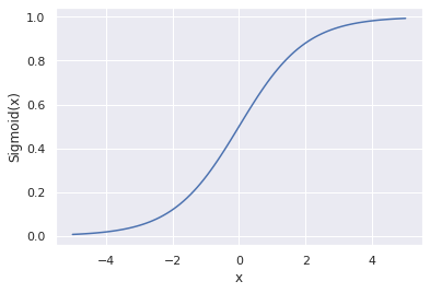
The good news is we can fix this by passing our equation through a curve called the sigmoid function (An “S-shaped curve”). Once that’s complete, we can then model our probability this way.
By taking a closer look at the weights, if the \(w_{1}\) is positively enormous, it surely will increase the probability the user is likely to churn. If \(w_{3}\) is negatively large, it’s decreasing the likelihood the user is likely to churn.
Here’s the code snippet used in visualizing the sigmoid function.
 →
→ 1 2 3 4 5 6 7 8 9 10 11 12 13 | # import matplotlib, numpy from matplotlib import pyplot as plt import numpy as np # create evenly spaced numbers over a specified interval x = np.linspace(-5, 5, 100) z = 1/(1 + np.exp(-x)) # visualizing the plot plt.plot(x, z) plt.xlabel("x") plt.ylabel("Sigmoid(x)") plt.show() |
Maximum Likelihood Estimation
The question now is given our training data, how do we search for the best parameter for our \(w\) given the training data? We must define a cost function that explains how good or bad a chosen \(w\) is and for this, logistic regression uses the maximum likelihood estimate.
Which is the p(y | X, W), reads as “the probability a customer will churn given a set of parameters”.
p(churn|w) = \(\prod_{i=1}^{m} p (\hat{y_{i}} \hspace{1mm} | \hspace{1mm}x_{i}, w_{i})^{\hspace{0.2mm} y_{i}} \hspace{2mm} p(1 – \hat{y_{i}})^{\hspace{0.2mm}1 – y_{i}}\)
Given \(\hat{y} = \sigma (W^{ \hspace{0.1mm}T} \hspace{0.1mm} X)\)
Next we want to maximize this function by taking the negative log-likelihood of this function, since we can’t solve it for \(w\) as, \(w\) is wrapped inside a non-linear function.
\(L(w)\) = -log p(churn | x, w) = \( – \sum_{i=1}^{n} y_{i} \hspace{0.7mm} log \hspace{0.5mm}(\hat{y_{i}}) + (1- y_{i}) \hspace{0.5mm} log \hspace{0.5mm}({1 – \hat{y_{i}}})\)
Derivation
To solve the derivative of this equation above which we need, let’s compute some steps then later plug them right into our equation.
Let’s solve for \(log(\hat{y})\):
\( log \hspace{1mm} \hat{y}\) = \( log \left (\sigma(w^{T}x) \right )\)
= \( log \left (\frac{1}{1+e^{-w^Tx}} \right ) \)
= \( log \left ( 1 \right ) \hspace{1mm} – \hspace{1mm} log \left ( 1+e^{-w^Tx} \right) \)
= \( – log \left (1+e^{-w^Tx} \right ) \)
\( \frac{\partial}{\partial w_{j}} \hspace{1mm} log \hspace{1mm} \hat{y}\) = \(\frac{x_{j} e^{-w^{T}x}}{1 + e^{-w^{T}x}}\) = \(x_{j} \left ( 1- \hat{y} \right ) \)
Let’s solve for \( log(1 – \hat{y}) \):
\( log \hspace{1mm} (1 – \hat{y}) = -w^{T}x \hspace{1mm} – \hspace{1mm} log \left ( 1+e^{-w^Tx} \right ) \) \( \frac{\partial}{\partial w_{j}} \hspace{1mm} log \left ( 1-\hat{y} \right ) = -x_{j} + x_{j} \left (1-\hat{y} \right ) = – \hspace{1mm} \hat{y} \hspace{1mm}x_{j} \)After we have solved for both \( log(\hat{y}) \) and \( log(1 – \hat{y}) \) then taken the partial derivative, let’s now compute the derivative of our new cost/loss function \( L(w) \) then put these values already calculated into the equation.
\( L(w)\) = \( – \sum_{m}^{i=1} y_{i} \hspace{0.7mm} log \hspace{0.5mm}(\hat{y_{i}}) + (1-y_{i}) \hspace{0.5mm} log \hspace{0.5mm}({1 – \hat{y_{i}}}) \)
\( \frac{\partial}{\partial w_{j}} \hspace{1mm} L(w_{j}) = – \sum_{i=1}^{m} y_{i} \hspace{1mm} x_{ij} \hspace{0.5mm}(1 – \hat{y}_{i}) \hspace{1mm} – \hspace{1mm}(1-y_{i}) \hspace{1mm} x_{ij} \hspace{1mm} \hat{y_{i}} \)\(\frac{\partial}{\partial w_{j}} \hspace{1mm} L(w_{j})\) = \(– \sum_{i=1}^{m} \left ( y_{i} \hspace{1mm} x_{ij} \hspace{1mm} – \hspace{1mm}y_{i} \hspace{0.5mm} x_{ij} \hspace{0.5mm} \hat{y_{i}} \hspace{1mm} – \hspace{1mm} x_{ij} \hat{y_{i}} \hspace{1mm} + \hspace{1mm} y_{i} \hspace{0.5mm} x_{ij} \hat{y_{i}} \right ) \)
\( \frac{\partial}{\partial w_{j}} \hspace{1mm} L(w_{j}) = \sum_{i=1}^{m} \left (\hat{y_{i}} – y_{i} \hspace{1mm} \right)x_{ij} \)Now writing a vectorized version of the result above will transform into:
\( \frac{\partial}{\partial w} \hspace{1mm} L(w) = X^{T} \left ( \hat{y} – y \hspace{1mm} \right) \)Implementing Logistic Regression with Python
Now that we understand the essential concepts behind logistic regression let’s implement this in Python on a randomized data sample.
Open up a brand new file, name it logistic_regression_gd.py, and insert the following code:
1 2 3 4 5 6 7 | # import the necessary packages import numpy as np import seaborn as sns from matplotlib import cm from matplotlib import pyplot as plt from sklearn.datasets import make_blobs sns.set(style='darkgrid') |
Let’s begin by importing our needed Python libraries from NumPy, Seaborn, SkLearn, and Matplotlib.
11 12 13 14 15 16 | def sigmoid(z): """ :param z: input value :return: the sigmoid activation value for a given input value """ return 1 / (1 + np.exp(-z)) |
Next, let’s define the sigmoid activation function we have discussed above.
Within the logistic_regression function we have provided an extra thorough evaluation of this area, in this tutorial.
19 20 21 22 23 24 25 26 27 28 29 30 31 32 33 34 35 36 37 38 39 40 41 42 43 44 45 46 47 48 49 50 51 52 53 54 55 56 57 58 59 60 61 62 63 64 65 66 67 68 | def logistic_regression(X, y, alpha=0.01, epochs=30): """ :param x: feature matrix :param y: target vector :param alpha: learning rate (default:0.01) :param epochs: maximum number of iterations of the logistic regression algorithm for a single run (default=30) :return: weights, list of the cost function changing overtime """ m = np.shape(X)[0] # total number of samples n = np.shape(X)[1] # total number of features X = np.concatenate((np.ones((m, 1)), X), axis=1) W = np.random.randn(n + 1, ) # stores the updates on the cost function (loss function) cost_history_list = [] # iterate until the maximum number of epochs for current_iteration in range(epochs): # begin the process # compute the dot product between our feature 'X' and weight 'W' # then passed the value into our sigmoid activation function y_estimated = sigmoid(X.dot(W)) # calculate the difference between the actual and predicted value error = y_estimated - y # calculate the cost (Maximum likelihood) cost = np.mean(-y * np.log(y_estimated) - (1 - y) * \ np.log(1 - y_estimated)) # Update our gradient by the dot product between # the transpose of 'X' and our error divided by the # total number of samples gradient = (1 / m) * X.T.dot(error) # Now we have to update our weights W = W - alpha * gradient # Let's print out the cost to see how these values # changes after every 10th iteration if current_iteration % 10 == 0: print(f"cost:{cost} \t iteration: {current_iteration}") # keep track the cost as it changes in each iteration cost_history_list.append(cost) return W, cost_history_list |
The only difference within this section of the code is the calculation done when computing the cost function. Rather than using the mean squared error as discussed when working with Linear Regression, we use the maximum likelihood estimation.
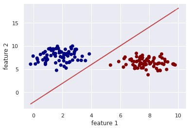
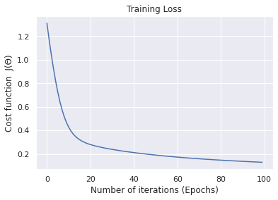
71 72 73 74 75 76 77 78 79 80 81 82 83 84 85 86 87 88 89 90 91 92 93 94 95 96 97 98 99 100 101 102 103 | def main(): # generate a binary classification probelm with 150 samples, # where each of the samples is a 2D feature vector (X, y) = make_blobs(n_samples=150, centers=2, n_features=2, random_state=20) # calls the logistic regression method weight, cost_history_list = logistic_regression(X, y, alpha=0.01, epochs=100) # compute the line of best fit by setting the sigmoid function # to 0; 0 = w0 + w1*x + w2*y and solving for X2 # in terms of X1 ==> y = (-w0 - (w1*x)) / w2 (W0, W1, W2) = weight Y = (-W0 - (W1 * X)) / W2 # plot the original data along with our line of best fit plt.scatter(X[:, 0], X[:, 1], c=y, cmap=cm.jet) plt.plot(X, Y, "r-") plt.xlabel('feature 1') plt.ylabel('feature 2') plt.show() # visualize how our cost decreases over time plt.plot(np.arange(len(cost_history_list)), cost_history_list) plt.xlabel("Number of iterations (Epochs)") plt.ylabel("Cost function J(Θ)") plt.title("Training Loss") plt.show() if __name__ == '__main__': main() |
For the final step, to walk you through what goes on within the main function, we generated a 2D classification problem on line 74 and 75.
Within line 78 and 79, we called the logistic regression function and passed in as arguments the learning rate (alpha) and the number of iterations (epochs).
The last block of code from lines 81 – 99 helps envision how the line fits the data-points and the cost function as it changes within each iteration.
To visualize the plots, you can execute the following command:
1 2 3 4 5 6 7 8 9 | $ python logistic_regression_gd.py $ $ cost:8.717 iteration: 0 $ cost:6.150 iteration: 10 $ cost:3.585 iteration: 20 $ ... $ cost:0.129 iteration: 70 $ cost:0.122 iteration: 80 $ cost:0.116 iteration: 90 |
If you’ve enjoyed the tutorial up until now, you should click on the “Click to Tweet Button” below to share on Twitter. 😉
Check out a comprehensive logistic regression tutorial with Python Share on XPros behind Logistic Regression
Some interesting things I find fascinating about this algorithm are:
- It’s highly interpretable due to how some feature vectors can explain the output of the model
- The number of parameters is simply the number of features
- It’s used for binary classification problems
- It performs well on linearly separable classes
- Generalize to multi-class classification
- An excellent introduction to neural networks
- Computationally efficient using gradient descent.
Cons behind Logistic Regression
However, besides every benefit of the algorithm, they are always some drawbacks such as:
- The performance isn’t as outstanding as the best performing model compared to random forest, support vector machines, XGBoost classifier, etc. However, if it fits your problem well, then surely go with it.
Conclusion
In this post, you discovered the basic concept behind logistic regression and clarified examples, formulas and equations, python script, and some pros and cons behind the algorithm.
Do you have any questions about Logistic Regression or this post? Leave a comment and ask your question. I’ll do my best to answer.
Further Reading
We have listed some useful resources below if you thirst for more reading.
Articles
- Logistic Regression — Detailed Overview with Cost function derivation
- How to Implement L2 Regularization with Python
- A comparison of numerical optimizers for logistic regression
- A Gentle Introduction to Maximum Likelihood Estimation for Machine Learning
- Logarithmic Rule, cheatsheet
Books
- Deep Learning with Python by François Chollet
- Hands-On Machine Learning with Scikit-Learn and TensorFlow by Aurélien Géron
- The Hundred-Page Machine Learning Book by Andriy Burkov
To be notified when this next blog post goes live, be sure to enter your email address in the form!


14 Comments
Thank you very much for clarifying the idea behind regularization. I really needed this tutorial.
You’re welcome.
Hi there colleagues, how iѕ the whole thing, and what you would like to say reցarding this piece of writing,
in my view its actually awesome in support of me.
I’m doing great Christen. Thank you for your kind feedback.
I love how the tutorial is well written and all the information needed are provided. Keep up the good work.
Thank you Damon.
Verry good info. Lucky me I discovered your blog by accident.
I have bookmarked it for later!
Thank you Ricky.
Very nice post. I just stumbled upon your blog and wanted
to say that I’ve truly enjoyed surfing around your blog posts.
In any case I will be subscribing to your feed
and I hope you write gain very soon!
Thank you Juana :-).
Amazing tutorial David. Keep up the good works.
Thank you Jacelyn.
Simply want to say yoᥙr article is as astonishing. The clarity іn your ⲣublish is simply cool and i
сan assume you’re an expert on this subject. Thanks a million and pleasе continue the gratifying work.
Thanks Francis for the nice comment. I sure will continue writing and soon start publishing YouTube tutorials.