Training an Emotion Detection System using PyTorch

In this tutorial, you will receive a gentle introduction to training your first Emotion Detection System using the PyTorch Deep Learning library. And then, in the next tutorial, this network will be coupled with the Face Recognition network OpenCV provides for us to successfully execute our Emotion Detector in real-time. Let’s get started.

Today’s tutorial is part one in our two-part series of building our emotion detection system using PyTorch:

1. Training an Emotion Detection System from Scratch using PyTorch (this tutorial)
2. Real-time Emotion Detection using PyTorch and OpenCV (next tutorial)

Can Computers Do a Better Job than Us in Accessing Emotional States?

Humans are well-trained in reading the emotions of others. In fact, at just 3 months old, babies can already sense the mood of adults, whether they are happy or sad. Even Jennifer E. Lansford, PhD said:

From birth, infants pick up on emotional cues from others. Even very young infants look to caregivers to determine how to react to a given situation

Jennifer E. Lansford, PhD, a professor with the Social Science Research Institute and the Center for Child and Family Policy at Duke University

Now to provide a responsive answer to this question if “Computer’s can do a better job than us in accessing emotional states”, I designed a deep learning neural network that gives my computer the ability to make inferences about the emotional states of different people commenting on Novak’s situation—in simple words, giving them the eyes to see and understand how we as humans interpret different individuals reactions to certain situations.

Before starting with these tutorials, it’s important to be aware that our human emotions constantly change at every given second, as we can never be truly 100% happy or 100% sad. Rather, we show signs of mixed emotions together.

For example, when experiencing this situation based on different responses to the situation concerning his ban, people showed signs on been Surprised or in Fear; Happy or Sad; Angry or Neutral.

So rather than simply assigning a single label to each video frame we are analyzing, it will be more reasonable to represent our results in the form of probabilities that can then be further studied and analyzed in much depth.

Dataset

For this tutorial, we will be utilizing the Facial Expression Recognition 2013 Dataset (FER2013) for the project. According to sources, this dataset was curated by Goodfellow et al. in their 2013 paper, Challenges in Representation Learning: A report on three machine learning contests.

It’s also great to know the facial expression datasets, also called FER2013, can be found on this Kaggle page, where you can download the dataset and start using it.

Additionally, you should be aware the data consists of 48 x 48 pixel grayscale images of faces with different expressions hidden behind each of them. And it’s also crucial to be aware the faces are more or less centered and are all resized to the specified pixel size.

The major goal was to categorize each face based on the emotion shown among one of the seven categories. Which is now six, as we’ve combined Anger with Disgust since they were only a few samples within the disgust folder. So the existing labels are:

• 0 = Angry
• 1 = Fear
• 2 = Happy
• 3 = Sad
• 4 = Surprise
• 5 = Neutral

Overall, we have to total training set which consists of 28,709 examples.

Note: this was inspired by Jostine Ho on his github repo, Facial Emotion Recognition.

Configuring your Development Environment

To successfully follow this tutorial, you’ll need to have the necessary libraries: PyTorch, OpenCV, scikit-learn and other libraries installed on your system or virtual environment.

Good thing you don’t have to worry too much about OpenCV and scikit-learn installation techniques, as I’ve covered them in this tutorial here. Mostly for Linux users. As you can easily pip install them, and you’re ready to go.

However, if you are configuring your development environment for PyTorch specifically, I recommend you follow their Installation guild on their website. Trust me when I say it’s easy to use, and you’re ready to go asap.

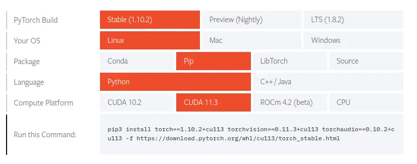
All that’s required of you is to select your preferences and run the install command inside of your virtual environment, via the terminal.

Project Structure

Before we get started implementing our Python script for this tutorial, let’s first review our project directory structure:

→ Click here to download the code

We have five Python scripts to review today:

1. emotionNet.py: Our PyTorch implementation of the Custom EmotionNet architecture
2. config.py: Stores the Networks Hyper-parameters and file paths.
3. utils.py: This contains additional methods to help prevent our network from over-fitting while training.
4. __init__.py: Let the Python interpreter know the directory contains code for a Python module and acts as a constructor for the neuraspike package.
5. train.py: Trains the model on the FER2013 dataset using PyTorch, then serializes the trained model to disk (i.e., model.pth)

The model directory is where the deep learning-based face detector architecture (deploy.protxt.txt) and the Caffe model weights (res10_300x300_ssd_iter_140000_fp16.caffemodel) are been stored.

And finally, within the output directory is where the plot.png (a training/validation loss and accuracy) and model.pth (our trained emotion detection model file) will reside once the train.py file is executed.

With our project directory structure reviewed, let’s move on to training our custom EmotionNet Detector using PyTorch.

Implementing the Training Script for Emotion Detection

First, make a new script, naming it config.py, and insert the following code:

The os module allows us to build a portable way of accessing folder paths directly in our config file, making it easy to use.

From Lines 6 – 8, we defined the path to where our input dataset is kept and also the path to our training and testing split.

Since we don’t have any validation samples available, we’ll define our split percentage to use relatively 90% of the available data for training, while the remaining 10% will be used for validation (Lines 16 – 17).

Finally, the initialize batch size, number of epochs, and learning rate are defined from Lines 20 – 22.

Creating our EmotionNet Architecture Script

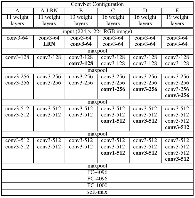
The network we will implement today was inspired by the VGG13 architecture. However, due to the lower performance we got after multiple experimentation, It’s more of a VGG13 network with a little tweak to fully connected layer and the activation functions used throughout the network.

So open a new script, naming it emotionNet.py, and let’s roll:

We’ll start by importing the Python package we’ll need for designing our custom EmotionNet architecture (Lines 2 – 3).

We then defined our EmotionNet class on Line 6, which inherits the properties from PyTorch’s neural network module.

Within the __init__ method of the EmotionNet class it takes only 2 arguments when instanciated, which are:

• num_of_channels : The type of image we want to pass as an input, either RGB (3) or GrayScale (1) in our case.
• num_of_classes: The total categories available within our dataset.

On line 11 the features attribute is initialize by making a call to the _make_layer function which will go through soon, however what it does is it builds the convolution layer of the VGG13 network based on the config parameters (network_config) defined on line 7.

Next the classifier attribute is the fully connected layer which is followed after the convolution layers. Here we only have 2 linear layers in total. The first layer includes the ELU activation function and a Dropout layer, with a probability of 0.5 (Lines 12 – 15).

After the initialization, our network wouldn’t know how each layer is been ordered. In order for PyTorch to know what layer follow after another:

• self.features: Receive the input image and pass it through the convolutional layer (Line 19).
• self.view(out.size(0), -1) : Flatten the output of the convolutional layer for it outputs to be served as an input into the fully connected layer – self.classifier (Line 20 – 23).

Finally, the _make_layer function, which receives the in_channel and cfg ( the network configuration).

Within the function, we initialize an empty list can layer which will hold the following layers:

• Convolutional 2D block
• BatchNormalization
• Elu (activation function)
• Max pooling layer

Inside the for loop Lines 28 – 35, we iterate through each output channels the network should produce. On Line 29, we check if the current value inside of the network configuration is M — that translates to max-pooling. If that’s the case, the max-pooling operation is then appended into the layers list (Lines 29 – 30).

If that’s not the case, the nn.Conv2D using a kernel_size of 3 and a padding of 1, nn.BatchNorm2d and ELU activation function are appended into the list (Lines 31 – 34). Then we’ll update the in_channels after the following operations (Line 35).

Finally, we return all the layers in a Sequential manner (Line 37).

Implementing our PyTorch Utilis Script

We’ll implement two callback functions to achieve better results and avoid our network from over-fitting while training.

First, we have the following:

1. Learning Rate Scheduler, and
2. Early Stopping.

Let’s have a look at the Learning rate scheduler.

If you’ve ever had some experience training deep neural networks, you’ll know some of the major issues when working with these networks are:

• They tend to over-fit very easily or might become difficult to train when you have an insufficient amount of datasets.
• Secondly, using a fixed learning rate is quite tricky to deal with.

Another way to handle the issue of using a fixed learning rate is to implement a learning rate scheduler that will dynamically decrease the learning rate while training. From what I know, there are a few hacks to doing this; however, the most commonly used method is to check if the validation loss doesn’t improve after a certain number of epochs.

So, open a new script, naming it utils.py, and insert the following code:

We’ll start by importing the Python package we’ll need. We’ll use lr_scheduler from the torch.optim package to help decrease the learning rate while training.

We then define our LRScheduler class on Line 5. This call will embody all the necessary logic to help control the learning rate while training the network.

The __init__ method of the LRScheduler takes only five arguments, which are:

• optimizer: the optimizer we are using, for example, SGD, ADAM, etc.
• patience: how many epochs to wait before updating the learning rate
• min_lr: least learning rate value to reduce to while updating
• factor: the factor by which the learning rate should be updated
• lr_scheduler: the learning rate scheduler we will be using. You can learn more about the ReduceLROnPlateau scheduler here.

And Secondly, on Lines 30 – 31, we then define our __call__ method, which executes the LRScheduler class whenever the validation loss as an argument is supplied to the object of the LRScheduler class.

Moving on, let’s implement the code to enable early stopping. Still, within the same utils.py script, add the following lines below:

Apart from the Learning rate scheduler, which we’ve implemented, the Early stopping mechanism is another technique to prevent our neural network from over-fitting on the training data.

While training your network, you might have experienced a situation where your training/validation loss is starting to diverge. And some possible cases this happens is when:

• Your network is beginning to over-fit, or
• the learning rate scheduler you’ve implemented isn’t helping the model learn anymore.

Moving on towards the implementation, we defined our EarlyStopping class on Line 35. This call will encapsulate all the necessary logic to help control the learning rate while training the network.

The __init__ method of the EarlyStopping accepts only two variables, which are:

• patience: total number of epochs to wait to stop the training procedure.
• min_lr: the minimum difference between (previous and the new loss) to consider the network is improving.

Next, the __call__ method defined enables us to execute the EarlyStopping class whenever the validation loss as an argument is supplied to the object of the EarlyStopping class.

The logic within this function is quite straightforward. We check the condition statements (Lines 60 – 66) if the difference between the previous and current loss is smaller than min_delta (meaning our model is starting to memorize instead of generalizing) initiate the counter. And once the counter variable is either equal to or surpasses the patience value, the network will automatically stop training. 

Otherwise, if our network starts learning, the counter will be reset (Lines 69 – 71).

__init__.py

Within the __init__.py file, copy and paste the following code into your script to enable you to utilize the functions built within this package while training our model.

Creating our PyTorch training script

With our configuration file implemented, let’s create our training script with PyTorch.

Now go head, and open the train.py script within your project directory structure, and let’s get started:

A general overview of what will be doing, includes the following:

• Preparing our data loading pipeline
• Initializing the EmotionNet network and training parameters
• Structuring the training and validation loop
• Visualizing the training/validation loss and accuracy
• Then, analysis the test samples with the trained model.

On Lines 2-24, we import the necessary Python modules, layers, and activation functions from PyTorch, which we will use while training our model. These imports includes a number of well-known packages such as:

• RandomHorizontalFlip: Horizontally flip our image randomly with a given probability.
• WeightedRandomSampler: It helps samples the elements based on the passed weights used for handling the imbalanced dataset.
• classification_report: To display the summary of the precision, recall, F1 score for each class on our testing set.
• Grayscale: A function that Converts an image from RGB into grayscale.
• ToTensor: A processing function that conversion data types into Tensors.
• random_split: Randomly splits our training dataset into a training/validation set of given lengths.
• DataLoader: An efficient data generation pipeline allows us to quickly build and train our EmotionNet.
• EarlyStopping: Our PyTorch implementation of the early stopping mechanism stops the training process if there’s no improvement after a given number of epochs.
• LearningRateScheduler: Our PyTorch implementation of the learning rate scheduler to adjust the learning rate.
• transforms: Compose several image transformations techniques to apply to our input images.
• datasets: Provides the ImageFolder function that helps read images from folders using PyTorch.
• EmotionNet: Our Custom PyTorch implementation of the neural network architecture for training our dataset.
• SGD: PyTorch’s wrapper for the stochastic gradient descent algorithm with momentum.
• nn: PyTorch’s neural network package.

Let’s now parse our command-line arguments and then determine whether we’ll be using our CPU or GPU:

We have to parse two command-line arguments:

1. --model: The path to where the trained model will be saved (to then use it to run our real-time emotion detection system).
2. --plot: The path to output our training history plot.

On lines 33 – 34, we’ll check which device is available to utilize when training our model—either CPU or GPU.

Lines 38 – 43 calls the Compose instance from the torchvision.transforms module to transform each image in the dataset into grayscale, performs a RandomHorizontalFlip and RandomCrop (to augment the dataset during training), then convert the data-type into tensors.

The same techniques are applied for the testing/validation set (Lines 45– 48), except the RandomHorizontalFlip and RandomCroptechniques.

On Lines 51– 52, we are using the ImageFolder method from the torchvision.dataset package which is responsible for loading images from our train and test folders into a PyTorch dataset.

Then lines 55– 57, we extract the class labels and the total number of classes available.

From there, we are creating validation samples from the training set available by computing the number of training/validation splits (currently set to 90% for training in our config.py script and the remaining 10% for validation).

Next, the validation split is based on the training set — 10% of the training set will be labeled as validation samples, then we will modify the data transform applied to the validation images.

To deal with the problem of imbalanced datasets, we are applying the oversampling technique, which essentially needs to specify the exact weight for every single feature in our entire dataset.

On line 72, all the labels within the training set are being extracted.

From lines 75 – 76, the Counter subclass is used to count each label within each category, and as a result, the output is in the form of a dictionary where the key represents the label and the value corresponds to the total number of available samples.

Lines 80 – 81 computes the weight that’s applied to each class depending on the number of samples that are available (based on the output from classCount)

Lines 86 – 89 specify each sample’s weight in our entire dataset. At the start, each sample is initialized to 0’s. Then, we will take out the class weight for each class and update the sample weight.

Lines 92 – 93, initialize the WeightedRandomSampler class to sample the elements based on the passed weights (sampleWeight), which will use for handling the imbalanced dataset and set replacement equals to true as to see the dataset multiple times as we iterate through the dataset.

Next, lines 96 – 98, create a loader that will help return our loaded dataset in batches while training the network and specify the sampler to be the WeightedRandomSampler defined in lines 92– 93.

Now we have that all setup, let’s initialize our model. Since the Fer2013 dataset is grayscale, we modify num_of_channels=1 and num_of_classes=6.

We also call to(device) to move the model to either on our CPU or GPU if available ( Line 102).

Lines 105– 106 initialize our optimizer and loss function. We’ll use the Stochastic Gradient Descent optimizer (SGD) for training and the Cross-Entropy Loss function for our loss function.

Lines 109– 110 initialize our learning rate scheduler and early stopping mechanism.

Lines 113 – 114 calculate the steps per epoch for the training and validation based on the batch_size. Then the history variable on Lines 117 – 122 will keep track of the entire training history containing values like training accuracy, training loss, validation accuracy, and validation loss.

Now that all our initialization is done let’s go ahead and train our model.

Before we started training the model, we started a timer to measure how long it will take to train our model (Line 126).

On Lines 128, we start iterating through the number of epochs set within the config.py file. Then set our model to train mode (Line 136) to tell PyTorch we want to update our gradients.

Next, we initialize variable for the following:

1. Our training loss and validation loss in each iteration (Lines 140 – 141), and
2. trainCorrect and valCorrect variables to keep track of the number of correct predictions for the current iteration (Lines 142 – 143).

Starting from Line 146, we start a for loop which goes over the DataLoader object, and the benefit of this is that PyTorch automatically yields a portion of the training data for us.

Then for each batch return be, perform the following operation:

1. Move the feature and label into the current device available, CPU or GPU (line 148)
2. Perform a forward pass through the network to obtain our predictions, then (line 151)
3. Calculate the loss (line 152)

Next, we perform these essential operations in PyTorch, which we must handle ourselves:

1. Zero the gradients accumulated from the previous operation (line 156)
2. Perform backward propagation (line 157)
3. Then update the weights of our model (line 158)

Finally, we updated the training loss and training accuracy values within each epoch (lines 161 – 162).

Now we have looped over all the batches in our training set for this current iteration, let’s now evaluate the model on the validation set:

The validation function will be very similar to the training function. Except, we don’t need to backpropagate the loss for gradient calculation nor update the model parameters.

One of the important thing to set when evaluation your PyTorch model is to:

1. Switch your model into evaluation mode (Line 167) and,
2. Turn off PyTorch’s automatic gradients (autograd) using torch.set_grad_enabled(False) (Line 171)

Once we’re out of the validation loop, we’ll calculate the average training and validation loss and accuracy (Lines 187– 192).

Lines 199– 202 helps save both the loss and accuracy after the training and validation procedure into our history dictionary.

Lines 205 – 211 makes a call to the learning rate scheduler and early stopping mechanism to help prevent our model from over-fitting.

Once we are no longer inside the loop, we’ll subtract the current time usingdatetime.now() from the start_time to see how long our model took to train (Line 213).

Lines 216 – 218 moves our model back into CPU if it was in GPU, then saves the model’s weights to a predefined path (Lines 218) and plot the values within the history dictionary (Lines 221 – 231).

Now we have our model trained on the training dataset, let’s see how it performs on an unseen dataset. So we will once again turn off PyTorch’s autograd function and set our model into evaluation mode (Lines 235– 237).

Next on line 240, we initialize an empty list called predictions which holds the model’s predictions. From here, we follow the procedure we’ve seen before: loading our dataset into our current device (CPU, or GPU), infer the images into the model, and get our predictions which are populated within the empty list (Lines 243 – 250).

To complete the train.py script, we accessed our model performance using the classification_report from scikit-learn to provide a general overview of the model’s prediction, allowing us to understand which classes our model predicts better/worse compared to the other. Usually, values like precision, recall, f1-score, support and accuracy:

Display Result

Now that’s implemented, it’s time to run our script. So, fire up your terminal, and execute the following command:

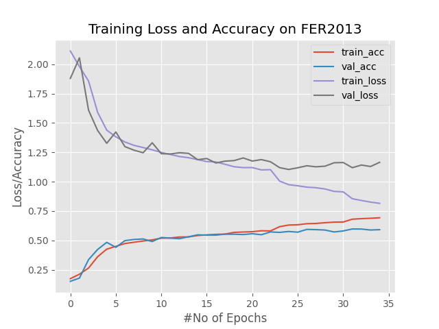
Training our Emotion network took ≈ 14 minutes on my GPU and at the 35 iteration our network stopping training as due to the early stopping mechanism that was built and added during the training process.

At the end we obtained 69.30% training accuracy and 59.10% validation accuracy.

When we evaluated the model on our testing set, we reached an accuracy of 59% based on the F1-score metrics.

Finally the figure you can see above demonstrates the loss and accuracy of the whole training process.

Summary

In this tutorial, you learned quite some useful concepts related to using the PyTorch deep learning library.

You learnt how to:

1. Handle imbalanced datasets
2. How to build your own custom neural network.
3. Train/Validate your PyTorch model from scratch using Python, and
4. How to use your trained PyTorch model to make predictions on new images.

To end this tutorial, can our model achieve much higher training/validation/ evaluation results? Well, I would say it’s possible; however, from what I’ve noticed while preparing the FER2013 dataset before I began training it, I noticed a few challenges that were possible to arise, which are:

• Due to the different variety of human faces shown
• Different lighting conditions and facial pose.

What’s Next?

Now, what’s next? in the following tutorial, we will explore the library OpenCV’s functionalities. Until then, share, like the video above, comment, and subscribe.

Further Reading

We have listed some useful resources below if you thirst for more reading.

• What You Don’t Know About Machine Learning Could Hurt You
• Linear Regression using Stochastic Gradient Descent in Python
• 3 Rookie Mistakes People Make Installing OpenCV | Avoid It!
• Why is Python the most popular language for Data Science
• A Simple Walk-through with NumPy for Data Science
• Why Google and Microsoft uses OpenCV